
I've recently been working on an internal project to predict future disk space usage for our customers across thousands of disks. Each disk is subject to its own usage patterns and this means we need a separate machine learning model for each disk which takes historical data to predict future usage on a disk-by-disk basis. While performing this prediction and choosing the correct algorithm for the job is a challenge in itself, performing this at scale has its own problems.
In order to take advantage of more sophisticated infrastructure, we can look to move away from sequential predictions and speed up the operation of the forecasting by parallelising the workload. This blog aims to compare Pandas UDFs and the 'concurrent.futures' module, two approaches of concurrent processing, and determine use cases for each.
The Challenge
Pandas is a gateway package in Python for working with datasets in the analytics space. Through working with DataFrames, we're able to profile data and evaluate data quality, perform exploratory data analysis, build descriptive visualisations of the data and predict future trends.
While this is certainly a great tool, the single-threaded nature of Python means it can scale poorly when working with larger data sets, or when you need to perform the same analysis across multiple subsets of data.
In the world of big data, we expect a bit more sophistication in our approach, as we have the additional focus on scalability to keep great performance. Spark, amongst other languages, allows us to take advantage of distributed processing to help us process larger and more complicated data structures.
Before digging into this specific example, we can generalise some use cases which summarise the need for concurrency in data processing:
- Apply uniform transformations to multiple data files
- Forecast future values for several subsets of data
- Tune hyperparameters for machine learning model and select most efficient configuration
When escalating our requirement to perform workloads like those suggested above and in our case, the most straightforward approach in Python and Pandas is to process this data sequentially. For our example, we would run the above flow for one disk at a time.
The Data
In our example, we have data for thousands of disks that show the free space recorded over time and we want to predict future free space values for each of the disks.
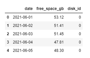
To paint the picture a bit more clearly, I've provided a csv file containing 1,000 disks each with one month of historical data for free space measured in GB. This is of sufficient size for us to see the impact of the different approaches to predicting at scale.
For a time-series problem like this, we’re looking to use historical data to predict future trends and we want to understand which Machine Learning (ML) algorithm is going to be most appropriate for each disk. Tools like AutoML are great for this when looking to determine the appropriate model for one dataset, but we’re dealing with 1,000 datasets here – so this is excessive for our comparison.
In this case, we’ll limit the number of algorithms we want to compare to two and see which is the most appropriate model to use, for each disk, using the Root Mean Squared Error (RMSE) as a validation metric. Further information on RMSE can be found here. These algorithms are:
- Linear regression
- Straight-line fitting graph used to model linear relationships.
- Fbprophet (fitting the data to a more complex line)
- Facebook’s time-series forecasting model.
- Built for more complex predictions with hyperparameters for seasonality.
We've got all the components ready now if we wanted to predict a single disk's future free space. The set of actions follows the below flow:
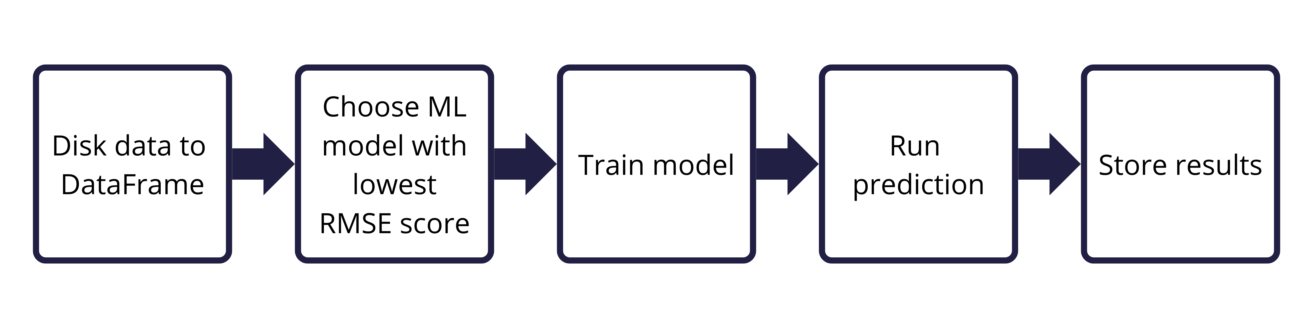
We now want to scale this out, performing this flow for multiple disks, 1,000 in our example.
As part of our review, we’ll compare the performance of calculating RMSE values for the different algorithms at different scales. As such, I’ve created a subset of the first 100 disks to mimic this.
This should give some interesting insights into performance on different-sized datasets, performing operations of varying complexity.
Introducing concurrency
Python is famously single-threaded and subsequently does not make use of all the compute resources available at a point in time.
As a result, I saw three options:
- Implement a for loop to calculate the predictions sequentially, taking the single-threaded approach.
- Use Python's futures module to run multiple processes at once.
- Use Pandas UDFs (user-defined functions) to leverage distributed computing in PySpark while maintaining our Pandas syntax and compatible packages.
I wanted to do a fairly in-depth comparison under different environment conditions, so have used a single-node Databricks cluster and another Databricks cluster with 4 worker nodes to leverage Spark for our Pandas UDF approach.
We’ll follow the following approach to evaluate the suitability of the Linear Regression and fbprophet models for each disk:
- Split the data into train and test sets
- Use the training set as input and predict over the test set dates
- Compare the predicted values with the actual values in the test set to get an Root Mean Squared Error (RMSE) score
We're going to return two things in our outputs: a modified DataFrame with the predictions, giving us the additional benefit of plotting and comparing the predicted vs actual values, and a DataFrame containing the RMSE scores for each disk and algorithm.
The functions to do so look like the below:
Setting up the experiment
We’re going to compare the three approaches outlined above. We’ve got a few different scenarios, so we can fill out a table of what we’re collecting results against:
| Method | Algorithm | Cluster mode | Number of disks | Execution duration |
|---|---|---|---|---|
| Sequential | Linear regression | Single node | 100 | |
| Concurrent.futures | Linear regression | Single node | 100 | |
| Pandas UDFs | Linear regression | Single node | 100 | |
| … | … | … | … |
With the following combinations:
Method:
- Sequential
- futures
- Pandas UDFs
Algorithm:
- Linear regression
- Fbprophet
- Combined (both algorithms for each disk) – most efficient way to gather a comparison.
Cluster mode:
- Single Node Cluster
- Standard Cluster with 4 workers
Number of disks:
- 100
- 1000
The results are presented in this format in the appendix of this blog, should you wish to take a further look.
The Methods
Method 1: Sequential
Method 2: concurrent.futures
There are two options in using this module: parallelising memory-intensive operations (using ThreadPoolExecutor) or CPU-intensive operations (ProcessPoolExecutor). One descriptive explanation of this is found in the following blog. As we're going to be working on a CPU intensive problem, ProcessPoolExecutor is fitting for what we're trying to achieve.
Method 3: Pandas UDFs
Now we're going to switch gear and use Spark and leverage distributed computing to help with our efficiency. Since we're using Databricks, most of our Spark configuration is done for us but there are some tweaks to our general handling of the data.
First, import the data to a PySpark DataFrame:
We're going to make use of the Pandas grouped map UDF (PandasUDFType.GROUPED_MAP), since we want to pass in a DataFrame and return a DataFrame. Since Apache Spark 3.0 we don't need to explicitly declare this decorator anymore!
We need to split out our fbprophet, regression and RMSE functions for Pandas UDFs due to DataFrame structuring in PySpark, but don't require a massive code overhaul to achieve this.
We can then use applyInPandas to produce our results.
Note: the examples above are only demonstrating the process for using Linear Regression for readability. Please see the full notebook for the complete demonstration of this.
Interpreting the results
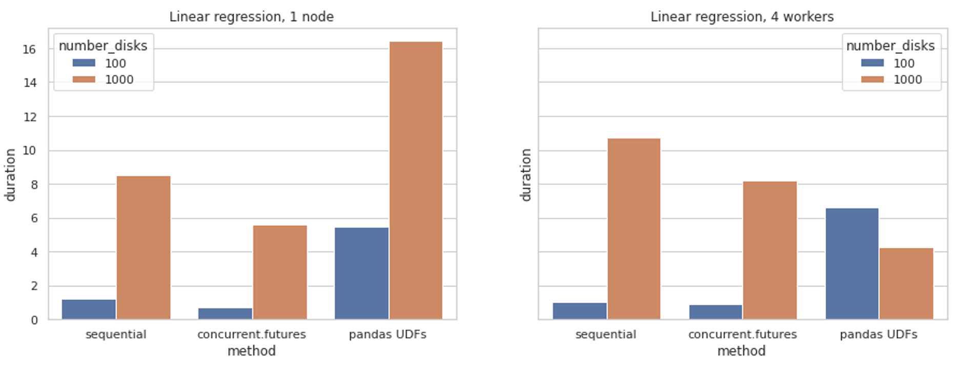
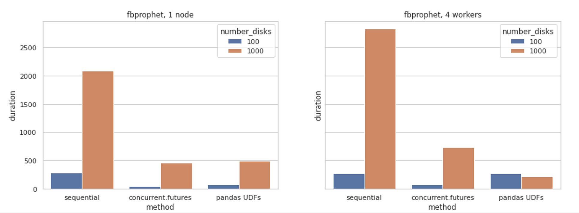
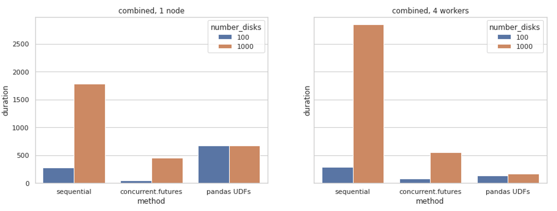
We’ve created plots for the different methods and different environment set-ups, then grouped the data by algorithm and number of disks for easy comparison.
Please note that the tabular results are found in the appendix of this post.
I’ve summarised the highlights of these findings below:
- As expected, predicting 1,000 disks compared to 100 disks is (generally) a more time-consuming process.
- The sequential approach is generally the slowest, being unable to take advantage of underlying resources in an efficient manner.
- Pandas UDFs are quite inefficient on the smaller, simpler tasks. The overhead of transforming the data is more expensive – parallelising helps to compensate for this.
- Both sequential and concurrent.futures approaches are oblivious to the clustering available in Databricks – missing out on additional compute.
Closing thoughts
Context certainly plays a big part in which approach is most successful, but given Databricks and Spark are often used for Big Data problems, we can see the benefit of using Pandas UDFs with those larger, more complex datasets that we’ve seen here today.
Using a Spark environment for smaller datasets can be done just as efficiently on a smaller (and less expensive!) compute configuration at great efficiency as demonstrated by the use of the concurrent.futures module, so do bear this in mind when architecting your solution.
If you’re familiar with Python and Pandas then neither approach should be a strenuous learning curve to move away from the sequential for loop approach seen in beginner tutorials.
We’ve not investigated it in this post as I have found discrepancies and incompatibilities with the current version, but the recent pyspark.pandas module will certainly be more common in the future, and one approach to look out for. This API (along with Koalas, developed by the guys at Databricks, but now retired) leverages the familiarity of Pandas with the underlying benefits of Spark.
For demonstrating the effect we are trying to achieve, we’ve only gone as far as to look at the RMSE values produced for each disk, rather than actually predict a future time-series set of values. The framework we’ve set up here can be applied in the same way for this, with logic to determine if the evaluation metric (along with other logic, such as physical limitations of a disk) is appropriate in each case and to predict the future values, where possible, using the determined algorithm.
As always, the notebook can be found in my GitHub.
Other posts related to the Coeo Disk Space Forecast can be found below:
https://blog.coeo.com/predictive-analytics-do-you-know-your-data
https://blog.coeo.com/new-disk-space-forecasting-available-for-dedicated-support
Appendix
| Method | Algorithm | Cluster mode | Number of disks | Execution duration |
|---|---|---|---|---|
| concurrent.futures | fbprophet | four workers | 100 | 74.46576 |
| sequential | combined | four workers | 1000 | 2842.584 |
| pandas UDFs | combined | four workers | 1000 | 167.5836 |
| sequential | fbprophet | four workers | 100 | 278.9985 |
| concurrent.futures | linear regression | four workers | 1000 | 8.201311 |
| pandas UDFs | fbprophet | four workers | 1000 | 216.7224 |
| sequential | fbprophet | four workers | 1000 | 2825.822 |
| pandas UDFs | linear regression | four workers | 100 | 6.583454 |
| concurrent.futures | combined | four workers | 100 | 75.55174 |
| sequential | linear regression | four workers | 100 | 1.026962 |
| pandas UDFs | combined | four workers | 100 | 130.7794 |
| concurrent.futures | linear regression | four workers | 100 | 0.914867 |
| pandas UDFs | fbprophet | four workers | 100 | 271.4759 |
| concurrent.futures | fbprophet | four workers | 1000 | 733.6325 |
| sequential | linear regression | four workers | 1000 | 10.7326 |
| concurrent.futures | linear regression | single node | 1000 | 5.582272 |
| sequential | combined | four workers | 100 | 288.2041 |
| pandas UDFs | linear regression | four workers | 1000 | 4.254914 |
| pandas UDFs | fbprophet | single node | 100 | 74.52466 |
| concurrent.futures | combined | four workers | 1000 | 554.86 |
| concurrent.futures | linear regression | single node | 100 | 0.710492 |
| pandas UDFs | linear regression | single node | 100 | 5.494357 |
| sequential | fbprophet | single node | 100 | 283.5356 |
| sequential | linear regression | single node | 100 | 1.241802 |
| sequential | linear regression | single node | 1000 | 8.498526 |
| pandas UDFs | combined | single node | 1000 | 672.0979 |
| pandas UDFs | linear regression | single node | 1000 | 16.40739 |
| pandas UDFs | fbprophet | single node | 1000 | 489.5573 |
| concurrent.futures | fbprophet | single node | 1000 | 457.6416 |
| sequential | combined | single node | 100 | 282.3154 |
| concurrent.futures | combined | single node | 1000 | 458.999 |
| concurrent.futures | fbprophet | single node | 100 | 49.05799 |
| sequential | fbprophet | single node | 1000 | 2088.575 |
| concurrent.futures | combined | single node | 100 | 48.04129 |
| pandas UDFs | combined | single node | 100 | 675.2854 |
| sequential | combined | single node | 1000 | 1785.651 |