
Machine Learning has become a buzzword for companies hoping to gain insights into future trends from historical behaviours. This leads to people associating predictive analytics with elaborate algorithms and difficult models, making it a complex and ambitious goal!
This doesn't always need to be the case. What if you could simplify your dataset, enabling you to pick a more straight-forward model that would in turn save you time, money and hours of work?
Machine Learning itself sounds sophisticated, but in reality it encompasses a wide variety of techniques to produce a result from your data. This could be a black-box solution such as a neural network, or something much simpler like linear regression. Both have their use-cases, but one is strikingly easier to understand, implement and de-bug.
Factors such as volume of data, anomalies, and changes in trends over time may sway your decision to pick the costly/elaborate tools – appealing as the more "robust" option.
Building your understanding
At this point, it is important to step back and understand the data we are currently dealing with in our data exploration of the "as is" dataset. By performing exploratory data analysis and understanding the trends and changes we can begin to understand the challenges a simplistic prediction/classification model might face.
- "These anomalies are due to this event last month."
- "This is business-as-usual behaviour that we need to account for."
- "We changed process A at time t, everything before that date is no longer representative of the current data."
- "Every 3 months another event takes place and we only want predictions including this."
- "We added another product category and the classification process needs to account for this."
These are all examples that show that we know our data and why it behaves the way it does. Without performing these data quality checks and grasping this knowledge, we may miss the opportunity to perform some pre-processing which will simplify the data modelling required. This can reduce the need for expensive and complicated models, bringing the benefit of faster predictions for less cost while maintaining (and possibly improving) accuracy.
Adding some context
Recently, I’ve been investigating time-series forecasting in disk space usage. Storage disks are used for a variety of functions and in the SQL Server world we see disks dedicated to database data files, log files, backup files, etc.
Disks can be expanded, data can be cleaned up on an ad-hoc basis or through routine procedures. These are examples of various possible scenarios that could change baseline activity that may lead to inaccurate forecasting if not understood.
These are all vital pieces of domain knowledge that when factored into our modelling process can greatly improve the reliability of our model.
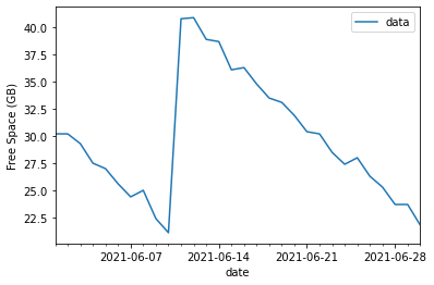
Take the example of a disk expansion. Plotting the data directly, we see the free space on the drive decreasing over time, with a sharp uptake in space on 2021-06-11 due to the expansion. After this event, the free space continues to decrease in a similar manner.
We could jump in and use a variety of models here, each with their own flaws in dealing with this untouched data. Consider Linear Regression and ARIMA models.
This is probably the most simple prediction model to understand as it looks to draw a linear relationship (when plotted, it forms a straight-line graph) for data points.
In our example, linear regression might expect the incorrect gradient in its straight-line prediction.
Autoregressive Integrated Moving Average (ARIMA):
This model is typically used in time series analysis where we see seasonality and other cyclical behaviours influence our data. It uses a combination of mathematical formula to reduce the data for easier predictions when dealing with variable and wave-like trends. Subsequently, this involves more model tuning and heavier computational requirements than a simple straight-line plot.
This model could expect that “jump” in disk space to be a cyclical pattern, and factor it into the prediction.
But we're smarter than this - we've got corresponding data elsewhere in our Data Warehouse that shows the drive size increasing by 20GB at this time. By performing some pre-processing in our modelling pipeline, we can acknowledge the expansion at this time, and adjust the data being passed into the prediction.
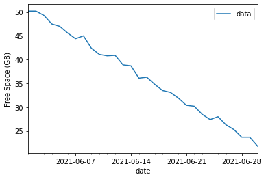
My approach in this case is to increase all values before the expansion event by 20GB, to compensate for this jump. The free space is still decreasing at the same increments, we’re just shifting our baseline.
We might also choose to use only data from after this event in our model, but working with a smaller dataset such as this could lead to less accurate predictions, with smaller test/training datasets.
Note: This is a manual demonstration of some data quality checks we could automate in our data cleansing pipeline.
Now look at the graph again - a (fairly) straight line, with a steady gradient before and after the expansion event:
Experience tells me that a simple linear regression algorithm should be able to handle this data with little error margin and be more accurate to future usage than without evaluating the expansion event beforehand. We can split the data into test and training samples to validate performance.
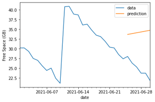
Comparing the two graphs, we can see the raw data leads to poor predictions – with the regression algorithm expecting the free space to actually trend upwards!
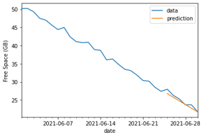
As you might expect, the steady gradient in our pre-processed dataset now gives a much better degree of accuracy we can predict against – which we can also validate mathematically by the improved Root Mean Squared Error (RMSE) metric. Now that we have some confidence in our model, we can start predicting future usage.
This is a simple example of how to apply exploratory data analysis and gain understanding of the "as-is" scenario, before jumping in and trying to build a model without seeing the story behind the data.
Closing thoughts
By taking the time to plot your data you can find and explain changes in patterns etc and ask the key question “Do you know your data?” needed to build the appropriate model and leverage your predictions.
If you’d like to a take a further look at this experiment, the code can be in the below repository: https://github.com/MattPCollins/LinearRegressionLab