
Slow-Running Query Due To Optimizer Timeout
I recently delivered a presentation at a SQL Server user group meeting where I presented a couple of interesting support cases. One of the cases I presented related to a slow-running query, which is something that all DBAs (and developers) should be able to instantly relate to.
Now, the problem about slow-running queries is that there are a multitude of possible reasons why a query may be running slow. However, what makes this particular case interesting (to me at least) is that the problem is easy to recognize just by looking at the query and the fix is easy to implement as well. It’s also surprising how often I come across the exact same problem, which would suggest that others must also experience this issue.
In this post I’ll describe the basic structure of the query and take a look at how the query optimizer works with a view to explaining why the query is slow-running. I’ll then discuss steps that you can take to avoid this specific problem.
The Query
To make this repeatable I’ve written a query that you can test yourself on AdventureWorks2012.
use AdventureWorks2012
go
select p.*
from Production.Product p
join Production.ProductProductPhoto ph on ph.ProductID = p.ProductID
join Production.ProductCategory pc on pc.ProductCategoryID = p.ProductSubcategoryID
join Production.WorkOrder wo on wo.ProductID = p.ProductID
join Production.WorkOrderRouting wor on wor.WorkOrderID = wo.WorkOrderID
join Production.Location l on l.LocationID = wor.LocationID
join Production.ProductModel pm on pm.ProductModelID = p.ProductModelID
join Production.ProductModelProductDescriptionCulture pmp on pmp.ProductModelID = pm.ProductModelID
left outer join Production.Culture c on c.CultureID = pmp.CultureID
left outer join Production.ProductDescription pd on pd.ProductDescriptionID = pmp.ProductDescriptionID
join Production.ProductDocument pdoc on pdoc.ProductID = p.ProductID
join Production.Document d on d.DocumentNode = pdoc.DocumentNode
join HumanResources.Employee e on e.BusinessEntityID = d.Owner
join Person.Person per on per.BusinessEntityID = e.BusinessEntityID
where <some predicates>
The above query is a fair representation of the type of query that I’m interested in demonstrating. Note that, for the purpose of testing this on a copy of AdventureWorks2012, you don’t need to worry about the WHERE clause and I’m using p.* for illustrative purposes only.
Also note that if you run the above query against AdventureWorks2012 it will run relatively quickly due to the low number of records that we’re dealing with. However, for the purpose of this post, it’s suitable for describing the problem.
The Execution Plan
If we run the above query with the Actual Execution Plan included it allows us to view the properties of the execution plan (click on the SELECT in the Execution Plan and press F4).
The Property window should look something like this:
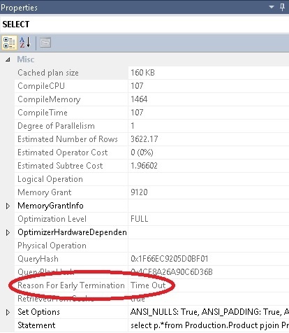
As we can see in the highlighted section the optimizer timed out whilst trying to obtain an execution plan. In order to describe what this means I will next explain the basics of how the query optimizer works.
The Query Optimizer
In simple terms the following flow diagram depicts the flow of tasks that the query optimizer goes through.
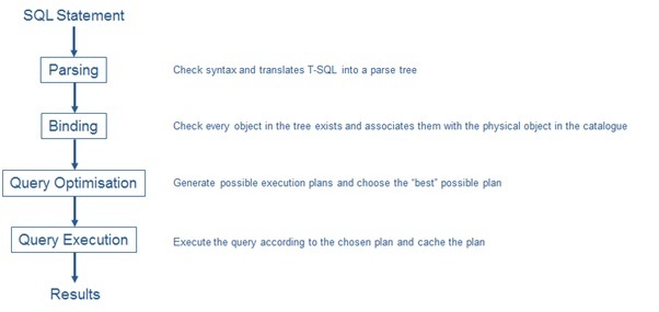
The section that I’m particularly interest in here is “Query Optimisation”. Here the optimizer needs to perform a number of steps which include:
- Compile a list of permutations of which tables to join and in which order
- Evaluate a number of join algorithms (i.e. loop, merge, hash)
- Evaluate a number of access methods (i.e. table scan, index scan, index seek, etc.)
- Evaluate aggregates and sub queries
- Estimate the cost of the possible plans
In this instance I would like to focus on the first of the above steps. This is where the optimizer compiles a list of permutations of which tables to join, and in which order.
To illustrate the task that is facing the optimzer let’s consider a simple example of two tables, involved in a join, as shown below.
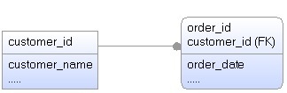
In the above example the optimizer can choose to join as follows:
- Customer Join Order; Or
- Order Join Customer
Both possible choices are equal in the sense that the resulting datasets produced will be identical (i.e. joining is commutative, like multiplication). However the order of joining is important and, depending on the sizes of the tables, one of the two options might be preferable.
Now, let’s complicate our simplified example by adding another table to the join, as shown below.
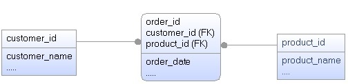
In the 3-table join shown above, the possible order permutations are as follows:
- (Customer Join Order) Join Product
- (Order Join Customer) Join Product
- Product Join (Customer Join Order)
- Product Join (Order Join Customer)
- Customer Join (Order Join Product)
- Customer Join (Product Join Order)
So with 3 tables there are 6 possible permutations that the optimizer has to evaluate.
In fact there are N factorial (N!) permutations, where N is the number of tables in the statement. With 10 tables there are 3, 628,000 possible permutations (10 x 9 x 8 x 7….. x 1).
For those of you that might not have noticed, there are 14 tables in the original query I used. This translates to over 86 billion permutations!
Think about this number for a moment and what it means. We’re asking the optimizer to evaluate 86 billion permutations and this is before it has even had a chance to perform steps 2-5 in the list of steps it needs to perform.
Note that, in reality, the problem is actually a bit worse than this but is beyond the scope of this post as the example I’ve used is sufficient to illustrate the scope of the problem. For those interested in further exploring this I recommend you start with exploring “deep left trees” and “bushy trees” in relation to the query optimizer.
As you might have guessed, the optimizer doesn’t actually evaluate this many permutations. Long before it gets to this point it gives up with the task at hand (hence the reason for early termination). What will happen is that the optimizer will have evaluated several thousand possible permutations prior to timing out and, at this point, will provide the “best” execution plan from that list. You may well be lucky and find that the optimizer has a chosen an execution plan that is decent. However, chances are that (statistically speaking) the execution plan that is chosen is not particularly good and can in fact be downright horrendous.
Help the Optimizer
As is hopefully obvious by now, the optimizer has a tough job on its hands and I consider our job (as DBAs and Developers) is to help the optimizer by making its job easier. The key thing to note is that the optimizer is not perfect and we need to do our best to give the optimizer the best possible chance of finding a good plan.
One of the best ways to help in this situation is to simplify the query by removing unnecessary joins or split up the single statement into several smaller statements. In a way this is analogous to how I like to approach all problem solving (split up problems into smaller, discrete problems).
Note that 6 or 7 joins is, ideally, the maximum number of joins the optimizer can cope with. This would correspond to around 700 or 5000 permutations respectively.
Simplifying the Query
As indicated, one of the approaches we can take is to simplify the query by splitting it up into smaller components. We can do this through the use of temporary tables as is illustrated below:
select p.*
into #temp1
from Production.Product p
join Production.ProductProductPhoto ph on ph.ProductID = p.ProductID
join Production.ProductCategory pc on pc.ProductCategoryID = p.ProductSubcategoryID
join Production.WorkOrder wo on wo.ProductID = p.ProductID
join Production.WorkOrderRouting wor on wor.WorkOrderID = wo.WorkOrderID
join Production.Location l on l.LocationID = wor.LocationID
select pm.ProductModelID
into #temp2
from Production.ProductModel pm
join Production.ProductModelProductDescriptionCulture pmp on pmp.ProductModelID = pm.ProductModelID
left outer join Production.Culture c on c.CultureID = pmp.CultureID
left outer join Production.ProductDescription pd on pd.ProductDescriptionID = pmp.ProductDescriptionID
select pdoc.ProductID
into #temp3
from Production.ProductDocument pdoc
join Production.Document d on d.DocumentNode = pdoc.DocumentNode
join HumanResources.Employee e on e.BusinessEntityID = d.Owner
join Person.Person per on per.BusinessEntityID = e.BusinessEntityID
select p.*
from #temp1 p
join #temp2 pm on pm.ProductModelID = p.ProductModelID
join #temp3 pdoc on pdoc.ProductID = p.ProductID
From the queries above we can see we have split our original single query into 4 queries. The first 3 queries are responsible for generating the data sets we’ll need, and the final query joins these 3 datasets to provide the output that would have effectively been returned by the original query.
If you examine the properties of each execution plan you’ll note that none of them have timed out.
It should be pointed out that in, literal terms, we are potentially asking SQL Server to do more work than it would have previously being doing. After all, whereas before it was running a single query, we’re now loading data into 3 separate temporary tables and then running a 4th statement against those temporary tables.
However, the cost of the original query using a bad execution plan is often far worse than the cost of doing a little bit of extra work.
In real terms I have applied this exact same approach with a customer where the original (20-join) statement was taking more than 24 hours to complete. After splitting up the single statement into 6 smaller statements, the multi-statement query was consistently finishing in under 20 minutes.
The last point about consistency is also quite important. When the optimizer times out it will choose the “best” plan amongst a list of several thousand; there is no guarantee that the next time a plan is chosen the same one will be chosen. I have seen several examples of large multi-table joins showing very inconsistent execution times (e.g. 20 hours one week and 10 hours the next week). So simplifying the query should also introduce consistency in ensuring that the same good plan is always chosen.
Summary
What I particularly like about this type of slow-running query is that it’s instantly obvious what the problem is. I don’t need to look at an execution plan or run the query; just count the number of tables in the statement. So whenever you see a query that has more than 6-7 joins in it consider whether you can help things along by simplifying it.
I should point out that simplifying the query is not the only option we have. For example we could use a plan guide (if we know a good plan) or we could force the join order by using query hints. However for the sake of keep things simple, I deliberately avoided discussing these other options in detail.
Even if simplifying the query doesn’t help produce a better plan, the act of simplifying it will help you troubleshoot the problem. When you have a number of statements to work with it’s easier to spot where the largest cost exists, as opposed to identifying the cost within a single statement that consists of 76 table joins. Believe it or not I have worked on a single select statement that had 76 joins in it!
In such a case, as a DBA, I think you’re perfectly within your rights to throw such a statement back at your developers and ask them to consider simplifying it – just a bit.
Update
I was recently asked whether it's possible to find query plans that are timing out on a SQL Server instance. At the time I hadn't thought to do this but I guessed that the query plan xml would probably be the best place to look. As it turns out, I was right and I was able to come up with the following query that returns the top 100 statements (and their plans) where query optimizer has timed out.
So not only do we have the means to fix this issue but we can now proactively go looking for it.
select top 100

quotename(db_name(qt.dbid)) as database_name

, quotename(object_schema_name(qt.objectid, qt.dbid)) + N'.' + quotename(object_name(qt.objectid, qt.dbid)) as qualified_object_name

, last_execution_time

, execution_count

, total_worker_time/1000.00/1000.00 as [total_cpu_time (seconds)]

, last_worker_time/1000.00/1000.00 as [last_cpu_time (seconds)]

, min_worker_time/1000.00/1000.00 as [min_cpu_time (seconds)]

, max_worker_time/1000.00/1000.00 as [max_worker_time (seconds)]

, (SELECT TOP 1 SUBSTRING(qt.text,statement_start_offset / 2+1 ,

( (CASE WHEN statement_end_offset = -1

THEN (LEN(CONVERT(nvarchar(max),qt.text)) * 2)

ELSE statement_end_offset END) - statement_start_offset) / 2+1)) AS sql_statement

, qp.query_plan

from sys.dm_exec_query_stats

cross apply sys.dm_exec_sql_text(sql_handle) as qt

cross apply sys.dm_exec_query_plan(plan_handle) as qp

where

charindex('StatementOptmEarlyAbortReason="TimeOut"', convert(nvarchar(max),qp.query_plan)) > 0

order by total_worker_time desc