Welcome to part three of the PDW Shallow dive. In this section I am going to explore partitioning in PDW. We will look at how to partition a table on the appliance and how to use partition switching. Unfortunately I was hoping to look at the CTAS function and specifically the mega merge statement but I will have to create a 4^th part of the series to cover that due to time constraints.

Introducing Partitioning on the PDW

Partitioning is used to help manage large tables. When partitioning a table you track logical subsets of rows with metadata. Unlike SMP SQL Server there is no partitioning function or scheme you simply set it when you create the table or use Alter Table to add partitioning to the table by selecting what column to partition by and setting your boundary values. This does not affect which distribution or compute node the data is stored on. Rather it will allow you to manage the table with these subsets of data, for example partition by month and then archive an older month by switching the partition to an archive table.

Let’s look at a simple example of a fact table that is partitioned, the code looks like this:

CREATE TABLE [dbo].[FactSales] (
[OnlineSalesKey] bigint NULL,
[DateKey] datetime NULL,
[StoreKey] int NULL,
[ProductKey] int NULL,
[PromotionKey] int NULL,
[CurrencyKey] int NULL,
[CustomerKey] int NULL,
[SalesOrderNumber] varchar(28) COLLATE Latin1_General_100_CI_AS_KS_WS NULL,
[SalesOrderLineNumber] int NULL,
[SalesQuantity] int NULL,
[SalesAmount] money NULL,
[ReturnQuantity] int NULL,
[ReturnAmount] money NULL,
[DiscountQuantity] int NULL,
[DiscountAmount] money NULL,
[TotalCost] money NULL,
[UnitCost] money NULL,
[UnitPrice] money NULL,
[ETLLoadID] int NULL,
[LoadDate] datetime NULL,
[UpdateDate] datetime NULL
)
WITH (CLUSTERED COLUMNSTORE INDEX, DISTRIBUTION = HASH([OnlineSalesKey]),
PARTITION ([DateKey] RANGE LEFT FOR VALUES (‘Dec 31 2006 12:00AM’, ‘Dec 31 2007 12:00AM’, ‘Dec 31 2008 12:00AM’, ‘Dec 31 2009 12:00AM’, ‘Dec 31 2010 12:00AM’, ‘Dec 31 2011 12:00AM’)));

It doesn’t have to be dates that are used to partition tables, although this is the most used option, you can partition tables by set values such a product categories or sales channels. Understanding the data you are working with and how it will be analysed is critical to set up partitioning. The key options for setting up partitioning are:

• The column – as mentioned before it is critical to identify the best column for partitioning your data by, in the example above we use the [DateKey] column.
• Range – this specifies the boundary of the partition, it defaults to Left (lower values) but you can choose Right (higher values), in the example above we use the default, Left. This means that the values specified will be the last value in each partition e.g. our first partition will have all data with a date before Dec 31 2006 12:00AM.
• The boundary value is the values in the list that you will partition the table by, this cannot be Null. These values must match or be implicitly convertible to the data type of the partitioning column.

Partitioning by example

In this section we will go step by step through a basic partitioning example. We create three tables, a main table with partitioning on it using a part_id, a second table used for archiving data from our main table and finally a table that we will use to move data from into our main table.

1. Create out our factTableSample with a partitioning option, using a part_id column:

   create table factTableSample

   (id int not null, col1 varchar(50),part_id int not null)

   with (distribution =
   replicate,
   partition(part_id range
   left
   for
   values(1,2,3,4,5)));
   

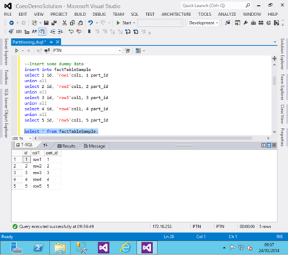
2. Now we will insert some basic data into the table:
   

   insert
   into factTableSample
   

   select 1 id,
   ‘row1′col1, 1 part_id
   

   union
   all
   

   select 2 id,
   ‘row2′col1, 2 part_id
   

   union
   all
   

   select 3 id,
   ‘row3′col1, 3 part_id
   

   union
   all
   

   select 4 id,
   ‘row4′col1, 4 part_id
   

   union
   all
   

   select 5 id,
   ‘row5′col1, 5 part_id
   

   Below shows what those rows then look like:
   

   
   

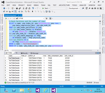
3. Let’s take a look at the how the data is stored in that table, how many rows are in each partition:
   

   –Check Paritions and the number of rows
   

   SELECT o.name, pnp.index_id, pnp.partition_id, pnp.rows,
   

   pnp.data_compression_desc, pnp.pdw_node_id
   

   FROM
   sys.pdw_nodes_partitions AS pnp
   

   JOIN
   sys.pdw_nodes_tables AS NTables
   

   
   ON pnp.object_id
   = NTables.object_id
   

   AND pnp.pdw_node_id = NTables.pdw_node_id
   

   JOIN
   sys.pdw_table_mappings AS TMap
   

   
   ON NTables.name = TMap.physical_name
   

   JOIN
   sys.objects
   AS o
   

   
   ON TMap.object_id
   = o.object_id
   

   WHERE o.name =
   ‘factTableSample’
   

   ORDER
   BY o.name, pdw_node_id, pnp.index_id, pnp.partition_id
   

   The results show that all but the final partition has 1 row in them. However you also notice there are 24 rows returned. This is because we created a replicated table that is replicated across our 4 nodes. For more information on replicated tables review part 1 of the series.
   

   
   

4. Now we will create an archive table to which we can move out older data:
   

   create
   table factTableSample_Archive
   (
   

   id int
   not
   null,
   

   col1 varchar(50),
   

   part_id int
   not
   null)
   

   with (distribution =
   replicate);
   

5. Now we can switch out partition 5 to the archive table and look at the results:
   

   alter
   table factTableSample switch partition 5 to factTableSample_Archive;
   

   
   

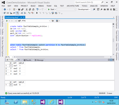
   We can clearly see that the 5^th partition has been moved from the main fact table (factTableSample) to the archive table (factTableSample_Archive).
   

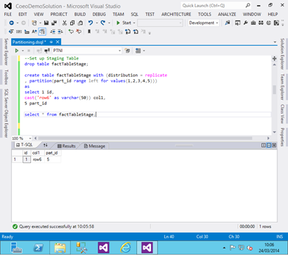
6. Next we create a new table which we would use to load staging data into:
   

   create
   table factTableStage with (distribution =
   replicate
   

   ,
   partition(part_id range
   left
   for
   values(1,2,3,4,5)))
   

   as
   

   select 1 id,
   

   cast(‘row6′
   as
   varchar(50)) col1,
   

   5 part_id
   

This adds a single row into partition 5:

1. Now let’s switch the stage data into partition 5 of the main fact table and look at the results:
   

alter
table factTableStage switch partition 5 to factTableSample partition 5;

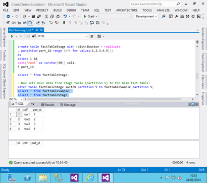
We see that partition 5 is now populated with the data from the stage table.

To summarise we can see using partitioning on the PDW is not overly complex. The alter table statements used to switch the partitions are very fast. If we had used distributed tables in the above examples it would have no effect on any of the code we used. Just like with SMP SQL Server it is important to plan your partitioning strategy in line with the analysis requirements and distribution of data in the datawarehouse. In the next part of the series I will dig into the CTAS (create table as select) statement and show an example of using this to do a merge into a dimension table. I hope you find the above useful, if you want any code examples please feel free to email at matt@coeo.com and I will get you a copy of the full script.