There is a very little amount of resource on the internet for PDW. I wanted to do a short series that will focus on the basics of PDW. I am not going into deep detail on the parallel engine or the commercial aspects, but instead am wanting to focus on what PDW is, where it sits in the Microsoft BI stack and what I found particularly useful as a Microsoft Business Intelligence specialist.
In part 1 of the series we will look at the following topics:
- Introduction to the PDW.
- PDW Exploration.
Introduction to PDW
So this is not a sales pitch but if you are looking at this blog you already see the value in having an eminently scalable and super performant datawarehousing appliance; in regards an idea of cost the current base offering from Microsoft comes in at around the cost of a high performance Fast Track Data Warehouse with tin and software licenses but for more info reach out to eddie@coeo.com who can help with any commercial questions around the PDW.
Ok so what is it?! Ultimately the PDW is an appliance – that’s it hope you liked it…
… Just kidding! It is an appliance that uses SQL Server 2012 (from v2). The appliance is really scalable by using SAN like technology and virtualisation software for redundancy. The appliance can be on either Dell or HP, both or any future hardware providers have to adhere to strict Microsoft guidelines and offer performance to a set level. In a way not dissimilar from the Fast Track Datawarehouse. In fact Microsoft learnt from all that work that went into recommending specific, optimum hardware for the fast track and built on that with the PDW appliance.
How does it differ from SMP SQL? Well with a single instance of SQL Server you get one buffer, one space for all your user requests (queries) to go through. This means that if one query is requested that user gets the whole buffer and it’s quick! However the more users requesting results or the more complex the queries then the buffer soon fills and users start having to wait.
With the PDW you get multiple instances of SQL Server working in parallel, meaning multiple buffers! User traffic can be managed by the management node to optimise performance. This MPP (Massive Parallel Processing) platform offers scalability, high concurrency, complex workloads and redundancy in a single appliance:
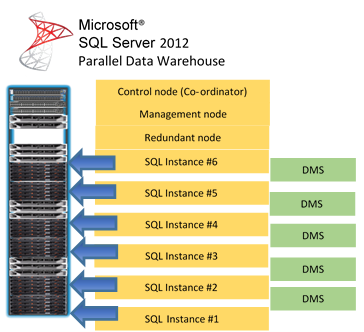
With the diagram example above we would have 6 SQL buffers to work with in parallel! The appliance comes in a single rack with a control node, management node and a load of SQL instances (depending on what variant of the appliance you buy); oh and there is also a redundant node for added failover should one of your nodes fail. The DMS is the data movement services, this is what controls how data is stored and moved on the various instances. More of this later.
PDW Exploration
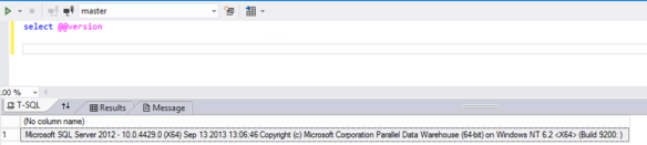
Ok so you know why you want one, let’s assume you get one, how do you go about developing on it? The first thing to note is that Microsoft has tried to make sure all the complexities of MPP are hidden from us. Ultimately we use our existing SQL Server and BI skills to develop against the appliance. To highlight this the graphic below shows that, once connected, the PDW is just seen as a slightly different version of SQL Server. It is good practice to use Visual Studio (and I find 2012 best at the moment) to work with the PDW.
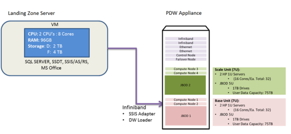
Now you don’t access the PDW directly on the management or control node. In your rack you will also have an SMP instance of SQL Server running on a Windows server, this is commonly called the landing zone or landing server. A typical architecture for a PDW rack may be:
To start work on the PDW we connect to the landing zone and then use Visual Studio Data Tools to connect to our server. For example it may look like:
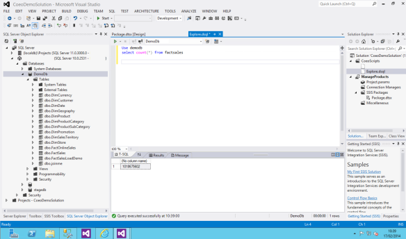
The next important concept you need is how you will store your data. There are two way to store your data. First is as distributed, so data is spread across all the SQL Server nodes. The second method is to store the data replicated. With this option the data will be copied to each SQL Server node. Because SQL Server still needs all the data on a single node to return the final results it uses the DMS (Data Movement Service) to move data around as it needs to complete a query. For smaller tables (generally dimension tables) it is best to use replicated so less DMS is needed. However for large fact tables it is much better to distribute that data so the PDW can apply the query across multiple nodes and use the processing power of each to get the queries and then pull that together to present the result. The diagram below shows a distributed fact table, by looking at the icon of the table in the SQL Server Object Explorer you can also see what is replicated and what is distributed:
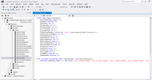
With distributed tables the important option is the key on which you want to distribute the data, above you can see we use OnlineSalesKey; to make the right choice it is critical to understand the data and also the potential use of the data, however it can be changed very quickly. This option will have the biggest bearing on performance of a distributed table. It is more important to use a key that has a balance of data volumes and is most used when querying the data. You will also notice above we use the Clustered ColumnStore Index (which is writeable) and we partition the table; we will talk more about both of these options in later blog posts.
The second option is replicated and you can see an example of a replicated table below:
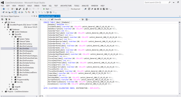
This will make our date dimension table replicated on all of the SQL Server nodes which will mean less DMS work so faster queries. Changing modes can be done easily and by using a PDW command called CTAS (Create Table As Select). You can quickly move data into a newly defined table; more on CTAS in later blog posts.
Finally in this section I wanted to show the central management portal for the PDW, this is a dashboard that can be accessed via the browser and an example is below:
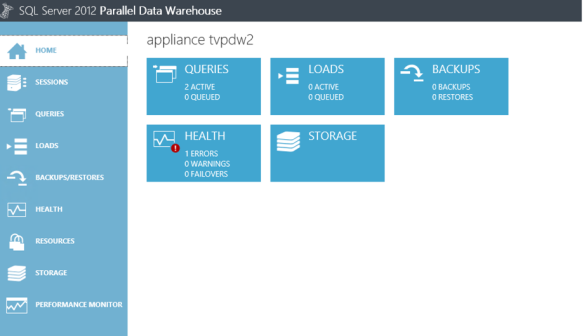
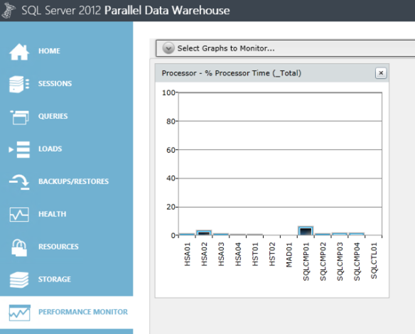
From this dashboard you will be notified of any potential issues with the appliance, note the red exclamation mark in the health section. It is also where you can look at query plans in detail to see how the PDW engine is managing the query. It is also a good place to monitor data loads, which we talk about in detail in part 2 of this series. Finally you can use the performance monitor to see what is happening in real time on your appliance, below shows an example of the performance monitor as I ran a Select * from dimFactSales that contains 10 million records. As it is distributed you see that all the SQL Server nodes are working at roughly the same time/levels:
So overall I hope I have shown you how relatively simple the PDW is. Under the covers we have a huge amount of impressive hardware and software that is optimised purely for datawarehouse loads yet above the covers we have our tried and tested SQL Server interface. My final thought in this part of my blog series is that with the PDW I suggest you have to slightly rethink your traditional BI strategy, for example using SSIS you don’t want to pull huge volumes of data from the PDW, manage them in the SSIS pipeline and then push them back onto the PDW, it is now much better to use SSIS as a control flow and let the PDW do more of the work. Also with regards the lack of a Merge statement, and the general ordinary performance of update statements it is critical to get used to being able to leverage the power of the PDW through the CTAS statement. In part 3 of this series I will expand on our mega-merge process which makes full use of the CTAS statement to update a dimension table with millions of records in seconds. I hope you like the start of this series and if you have any specific questions please leave a comment and I will endeavour to answer as soon as I can.

![]()